
The bias–variance tradeoff problem is the conflict in trying to simultaneously minimize the error that prevent supervised learning algorithms from generalizing beyond their training set:
Definiton
Suppose we want to estimate the parameters $ \theta $ which minimize a Cost function $ J(\theta) $ defined by the sum of all error across all samples between the prediction output $ \hat{y} $ and the expected output $ y $. This means, we have the expected value of $y = f(\theta , X) $ given $ X $ defined by $ \hat{y} = f(\hat{\theta}, X) $ and the estimated parameters:
$ \hat{\theta} = \theta + \epsilon $
This problem can be rewrited:
$ \hat{\theta} = \underset{\hat{\theta}}{argmin}$ $J(\theta) = \underset{\hat{\theta}}{argmin}$ $|| f(\theta, X) - f(\hat{\theta}, X)||^2 $
We know that the bias is how much predicted values differ from true values, and the variance is how predictions made on the same value vary on different realizations of the model and this result depends of $ \theta $ .
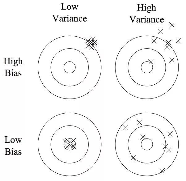
We deduce that the expected value of the error $ \mathrm{E}[\epsilon]=0$ , has some variance $ \mathrm{Var}[\epsilon]=\sigma^2_{\epsilon}$ .
In addition, we can calculate the Bias and the Variance of $ \hat{y} $ and $ y $ :
$ Bias_{\theta}[\hat{\theta}] = E[\hat{\theta} - \theta] = E[\hat{\theta}] - \theta $
$ \mathrm{Var}[\hat{\theta}] = E[( \hat{\theta} - E[\hat{\theta}])^2 ] = E[\hat{\theta}^2] - E[\hat{\theta}]^2 $
$ \mathrm{Var}[\theta] = E[( \theta - E[\theta])^2 ] = E[( \hat{\theta} - \epsilon - \hat{\theta})^2] $
$ \mathrm{Var}[\theta] = E[(\epsilon)^2] = \mathrm{Var}[\epsilon] + (E[\epsilon])^2 = \sigma^2_{\epsilon} $
So, we will determine the relation between Variance, Bias, and the error of the estimator parameter:
$ MSE(\hat{\theta}) = E[(\hat{\theta} - \theta)^2] = E[(\hat{\theta}^2 + \theta^2 - 2\theta \hat{\theta})] $
$ MSE(\hat{\theta}) = E[\hat{\theta}^2] + E[\theta^2] - 2 E[\theta \hat{\theta}] $
$ MSE(\hat{\theta}) = (\mathrm{Var}[\hat{\theta}] + E[\hat{\theta}]^2) + (\mathrm{Var}[\theta] + E[\theta]^2) - 2 E[\theta] E[\hat{\theta}] $
$ MSE(\hat{\theta}) = \mathrm{Var}[\hat{\theta}] + \mathrm{Var}[\theta] + (E[\hat{\theta}]^2 + E[\theta]^2 - 2 E[\theta] E[\hat{\theta}]) $
$ MSE(\hat{\theta}) = \mathrm{Var}[\hat{\theta}] + \mathrm{Var}[\theta] + (E[\hat{\theta}] - E[\theta])^2 $
$ MSE(\hat{\theta}) = \mathrm{Var}[\hat{\theta}] + \sigma_{\epsilon}^2 + (E[\hat{\theta}] - \theta)^2 $
$ MSE(\hat{\theta}) = \sigma_{\epsilon}^2 + \mathrm{Var}[\hat{\theta}] + Bias_{\theta}[\hat{\theta}] $
Overfitting/Underfitting Problems
When we are performing a parameter estimator $ J(\theta) $ , we could face to 2 scenarios:
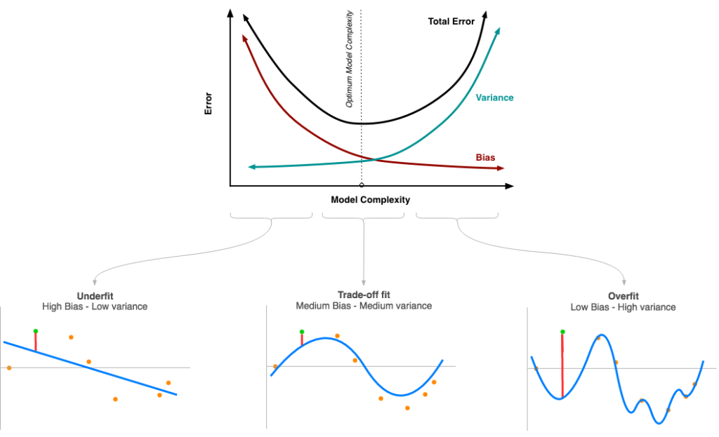
Underfitting (Bias error): (high bias, low variance, $ J({\theta}) \gt \gt 0 $ ) cause the algorithm to miss the relevant relations between features and target outputs.
Overfitting (Variance error): (low bias, high variance, $ J({\theta}) \approx 0 $ ) cause an algorithm to model the random noise in the training data, rather than the intended outputs.
Way to avoid this scenarios:
Feature selection or model selection algorithm.
Increase the sample size
Regularization
Regularization
Regularization is the process to prevent overfitting/underfitting by adding an additional penalty term in the error function.
Ridge (L2 regularizer)
LASSO (L1 regularizer)
Least Absolute Shrinkage and Selection Operator (LASSO) is quite similar conceptually to ridge regression. It also adds a penalty for non-zero coefficients. As a result, for high values of $ \lambda $ , many coefficients are exactly zeroed under lasso, which is never the case in ridge regression.
Elastic Net
Generalization
Be the norm-p defined as:
$ || \theta ||_p = \sqrt{\sum^m _{j=1} | \theta_i |^p} $
As we mention at the begining of this blog, supervised learning algorithms use to take the Ordinary Least Square (OLS) as a function error, let’s define the error for each sample as:
$ L(\hat{y}_i, y_i) = (\hat{y}_i - y_i)^2 $
So, adding the regularizer function $ R(\theta) $ to the Cost function defined above:
$ J(\theta) = \dfrac{1}{n} [ \sum ^n _ {i=1} L(\hat{y}_i, y_i) + R(\theta)_{\lambda,\alpha} ] $
$ R(\theta)_{\lambda,\alpha} = \lambda [ \dfrac{(1-\alpha)}{2} || \theta ||_2 + \alpha || \theta ||_1 ] $
Where:
- $ f $ is the estimator function.
- $ X \in \mathbb{R}^{nxm} , y \in \mathbb{R}^{n} $ is the data sample.
- $ {x}^i $ is one sample, $ x_j $ is one feature and $ {x_j}^i $ is the j-th feature in sample i.
- $ \theta = (\theta_1, \dots, \theta_m ) \in \mathbb{R}^{m} $ are the parameters.
- $ \hat{y} \in \mathbb{R}^{n} $ is the predicted output.
- $ n $ is the sample size.
- $ m $ is the number of features.
- $ \lambda \in \mathbb{R} $ regularization parameter, where $ 0 \lt \lambda \lt \inf $ .
- $ R_{\lambda} $ regularization equation with $ \alpha \in [0, 1] $ :
- If $ \alpha = 0 $ , then we have Ridge Regression.
- If $ \alpha = 1 $ , then we have LASSO.
- If $ 0 \lt \alpha \lt 1 $ , then we have Elastic Net.
Normal Equation
If m > n:
$ \theta = (X^T X + \lambda R) X^T y $
Else is Non-invertible. Also, R is:
$ R = \begin{bmatrix} 0 & 0 & 0 & \dots & 0 \\ 0 & 1 & 0 & \dots & 0 \\ 0 & 0 & 1 & \dots & 0 \\ \vdots & & \ddots & & \vdots\\ 0 & 0 & 0 & \dots & 1 \end{bmatrix} $
With:
$ R \in \mathbb{R}^{(n+1)x(n+1)} $